With my first guitar, I also got my first guitar tuner, a device that I have mixed feelings about. I can’t tune my guitar without it, but the tuner exposes just how fickle the concept of being “in tune” really is.
The author with his guitar, trying to look cool, circa 2021.
There are many reasons that it’s hard to tune your guitar, from the weather to number theory.1 This post adds another reason to this already long list:
The pitch of the note depends on how hard you pluck the string.
The effect is not subtle, and most experienced guitar players are well aware of the phenomenon. You can see it in the figure below where the peak-to-peak time drops as the amplitude increases, causing a hard pluck to go almost a quarter-tone sharp.
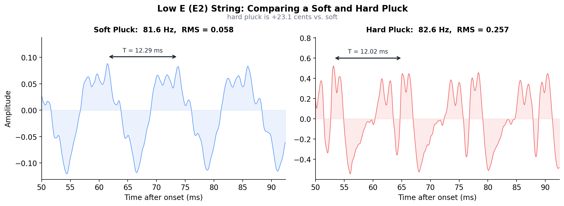
The low-E string plucked softly (left) and hard (right). The harder pluck is about a quarter tone sharp.
It’s easy to see the effect for yourself. If you have a guitar handy, try this simple experiment:
- Tune your low-E string with gentle picks, like normal.
- Without adjusting the tuning knob, increase the dynamics from piano to fortissimo.
- Watch the tuner go sharp as your notes get louder.
I recorded myself doing just this experiment, and then generated some code that extracts the notes and detects the pitch. Invariably, the loudest notes are quite sharp.
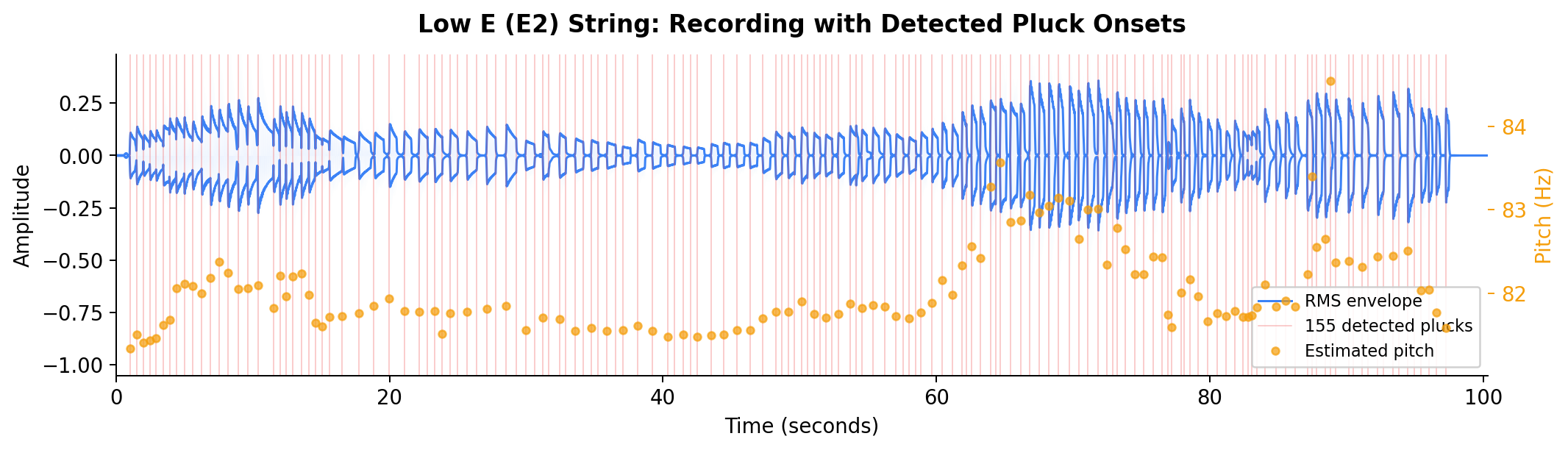
The low-E string on a guitar plucked at various intensities. The pitch has been extracted from each pluck and plotted on the y-axis.
What’s going on? The answer, as we’ll see below, is that the new resonant frequency of the string increases with the square of the amplitude of the pluck. With $\alpha$ as the amplitude of the pluck (in the appropriate units) and $f_0$ as the resonant frequency at a low amplitude:
$$ \frac{\Delta f}{f_0} \propto \alpha^2 \tag{1} $$For small amplitudes $\alpha \approx 0$, there is little change in pitch, but for modest to large amplitudes, the effect can be a dramatically sharp note. See the figure below. The low-E string on a guitar plucked at various intensities. We plot the RMS amplitude of the pluck against the pitch, and fit a quadratic curve.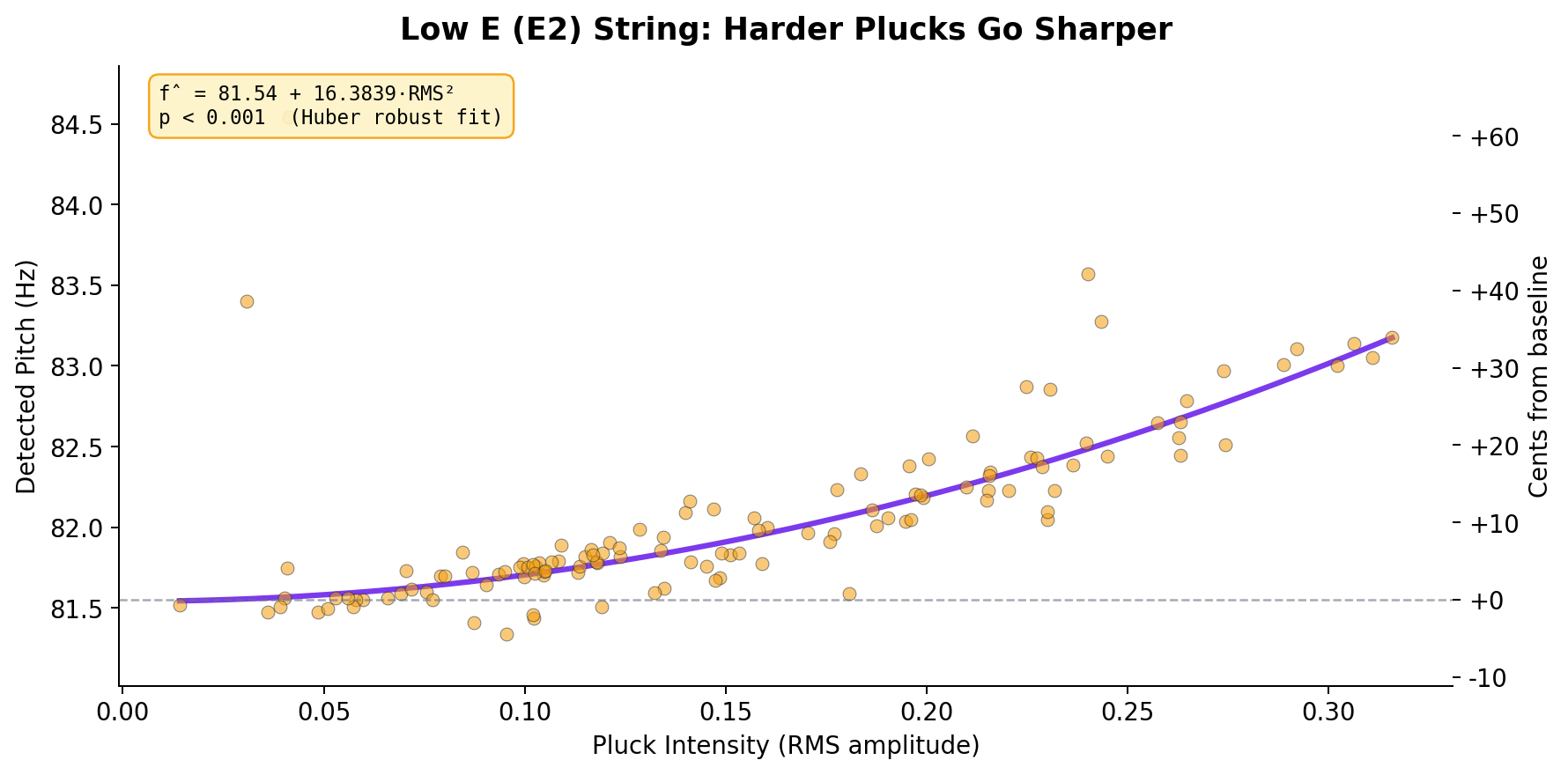
I’ll derive this relationship in detail below by studying a nonlinear PDE known as the Kirchhoff–Carrier equation.
Warning: The next bit is a math-heavy derivation involving nonlinear PDEs. If you aren’t up for that right now, skip ahead to the implications for musicians.
The physics of guitar strings
A guitar string is a stiff spring. When we tune a guitar we stretch this spring, pre-loading tension so that the string is always pulled back to its neutral resting position. The more tension in the string, the faster the string is pulled back. The inertia of the moving string causes overshoot, so the process repeats, creating a vibrating string, or tone.
Let’s model a vibrating guitar string as a height function $h(x,t)$ that describes how far the guitar string is displaced from its natural straight-line position at any given time $t$ and location along the string $x$. Then a well-known relation describes the vibrations along our string in terms of the tension $T$ along the string and the density $\rho$ (per unit length) of the string:
$$ \rho\, h_{tt} = T\, h_{xx}. \tag{2} $$This wave equation holds the key to our out-of-tune guitars. We begin with the assumption of constant tension $T = T_0$, which leads to the classical linear solutions of the wave equation.
Linear theory assumes constant tension
Assume for the moment that the tension $T=T_0$ is constant, independent of the displacement $h$. The easiest way to come up with a solution in this case involves what mathematicians call an ansatz and what everyone else calls “guess and check”. For every integer $n\ge 1$, we have one solution (aka harmonic) given by
$$ h_n(x,t) = \sin\left(\frac{n\pi}{L} x\right) \cos\left(\frac{n\pi}{L}\sqrt{\frac{T_0}{\rho}}t\right). $$The time-varying cosine term is of most interest to musicians, and the $n=1$ case yields the fundamental frequency
$$ f_0 = \frac{1}{2L} \sqrt{\frac{T_0}{\rho}}. $$The general solution is a superposition of these modes, i.e., $\sum_n \alpha_n h_n(x,t)$.
Vibration increases tension
A string displacement causes it to stretch slightly. A vibrating string is thus constantly changing its tension, even if just a little. To add this term to our tension model, consider the formula for the additional stretch of a displaced string locally:
$$ \mathrm{d}\ell - \mathrm{d}x = \sqrt{\mathrm{d} x^2 + \mathrm{d}h^2} - \mathrm{d}x \approx\frac{h_x^2}{2} \mathrm{d}x $$using a Taylor expansion. The additional tension from stretching equals $EA$ times the total fractional elongation of the string, where $E$ is the Young’s modulus and $A$ is the cross-sectional area. With the original tension $T_0$, the time-varying tension in our string is
$$ \text{Total tension} = T(t) = T_0 + \frac{EA}{2L}\int_0^L h_x^2 \mathrm{d}x, $$leading to the nonlinear Kirchhoff–Carrier2 wave equation
$$ \rho \,h_{tt} = \left( T_0 + \frac{EA}{2L}\int_0^L h_x^2 \mathrm{d}x\right) h_{xx}. \tag{3} $$Since $h_x^2 \ge 0$, the vibrating string is effectively tighter than in the simple linear string model. Let’s make this precise.
Reduction to a Duffing oscillator
To analyze the effect of the time-varying tension, we will study solutions of the form
$$ h(x,t) = \tau(t) \sin(\pi x/L). $$This ansatz (that word again!) can then be plugged into the Carrier equation above and we find an ODE for the time-varying function $\tau$:
$$ \ddot{\tau} + \omega_0^2 \tau + \gamma \tau^3 = 0 \tag{4} $$where
$$ \omega_0^2 = \frac{T_0 \pi^2}{\rho L^2}, \quad \gamma = \frac{EA \pi^4}{4\rho L^4}. $$This is a Duffing oscillator, and we’ll solve the problem using a well-known energy trick.
Solving the Duffing oscillator using energy
One of my favorite tricks is the energy method3 for analyzing ordinary and partial differential equations. Multiply (4) by the time derivative $\dot\tau$ and integrate from zero to $t$. After integration by parts, we find
$$ \frac{1}{2} {\dot \tau}^2 + \frac{\omega_0^2}{2} \tau^2 + \frac{\gamma}{4} \tau^4 = \mathcal{E} \tag{5} $$where $\mathcal{E}$ is the constant of integration that’s called the conserved energy; in particular, $\mathcal{E}$ does not depend on time.
Suppose that our maximum amplitude $\alpha$ of our vibrational mode $\tau(t)$ occurs at time $t=t^*$. Another way of saying this is $\tau(t^*) = \alpha$, $\dot \tau(t^*) = 0$, and $\ddot \tau(t^*) < 0$. Inserting into the energy relation (5), we find
$$ 2 \mathcal{E} = \omega_0^2 \alpha^2 + \frac{\gamma}{2} \alpha^4. $$From (4), we can also derive the inverse relationship between time and $\tau$:
$$ \frac{\mathrm d \tau}{\mathrm d t} = \sqrt{2 \mathcal{E} - \omega_0^2\tau^2 - \frac{\gamma}{2} \tau^4} \implies \frac{\mathrm d t}{\mathrm d \tau} = \left(2 \mathcal{E} - \omega_0^2\tau^2 - \frac{\gamma}{2} \tau^4\right)^{-1/2}. $$Graphically, $t^*$ is the time it takes to traverse the section of the phase space highlighted in red in the diagram below, so by symmetry $4 t^*$ is the total period of the wave.

Phase space of the Duffing oscillator. We integrate over the first quarter period to find $t^*$.
To compute $t^*$, we integrate from $\frac{\mathrm d \tau}{\mathrm d t}$ from zero to $\alpha$, use our formula for $2\mathcal{E}$, and make the inspired change-of-variables $\tau = \alpha \sin \theta$:
$$ t^* = \int_0^\alpha \frac{\mathrm d \tau}{\sqrt{2 \mathcal{E} - \omega_0^2 \tau^2 - \frac{\gamma}{2} \tau^4}} = \int_0^{\pi/2} \frac{\mathrm d \theta}{\sqrt{\omega_0^2 + \frac{\gamma\alpha^2}{2} (1+\sin^2 \theta)}}. $$Assuming that $\varepsilon := \frac{\gamma\alpha^2}{2\omega_0^2}$ is small, we can expand the square root to first order:
$$ t^* \approx \int_0^{\pi/2} \frac{1}{\omega_0} \left (1 - \frac{\varepsilon}{2} \left(1+\sin^2 \theta\right)\right)\mathrm d \theta = \frac{\pi}{2\omega_0} \left( 1 - \frac{3}{4}\varepsilon\right) $$Now tracing back our definition of $\varepsilon$ and $\gamma$ gives the new frequency $f := 1/4t^*$ in terms of our original frequency $f_0 := \omega_0 / 2\pi$:
$$ f \approx f_0\left(1 +\frac{3}{128} \frac{EA \pi^2}{\rho L^4f_0^2} \alpha^2\right). $$We’ve used the usual expansion $1/(1-x) \approx 1 + x$ for small $x$.
It’s helpful for interpretation to swap this into a different formulation. The linear density $\rho = \rho_{\mathrm{vol}} A$, where $\rho_{\mathrm{vol}}$ is the volumetric density. This allows us to cancel out the cross-sectional area $A$. Writing $\Delta f = f - f_0$, we are left with
$$ \frac{\Delta f}{f_0} \approx \frac{3\pi^2}{128} \frac{E\alpha^2}{\rho_{\mathrm{vol}}L^4 f_0^2}. \tag{6} $$This shows the claimed relation (1) above.
Implications for musicians
Generally speaking, guitar players will probably want to limit the dynamic range of their playing to stay in the “flat” regime. First and foremost, this means getting comfortable with the pitch-bending effects of dynamic range on each instrument, and adjusting your playing style accordingly. But changing physical parameters can also make a difference.
The relation from equation (6) above shows
$$ \frac{\Delta f}{f_0} \propto \underbrace{\left(\frac{\alpha}{L}\right)^2}_{\text{relative amplitude}} \times \underbrace{\frac{E}{\rho_{\mathrm{vol}}}}_{\text{material}} \times \underbrace{\frac{1}{L^2} }_{\text{string length}} \times \underbrace{\frac{1}{f_0^2}}_{\text{nominal frequency}} \tag{7} $$Let’s take these one at a time.
Relative amplitude
Amplitude is by far the easiest variable to adjust; most musicians have an intuitive feel for how hard they can pluck a string before the note begins to sound “off”. Lower amplitude leads to dramatically less pitch shifting. In our experiments, amplitudes up to roughly halfway to the maximum achievable yielded qualitatively acceptable tonal shifts.
In (7) above, we normalize the amplitude $\alpha$ by the length $L$ of the string to make a unitless quantity relative amplitude $\alpha/L$. This is the amount that the string displaces its center relative to its length. In normal playing, this ratio will likely be on the order of 0.1–1%.
Material
The material term includes the physical properties of the string: the Young’s modulus $E$ and the density $\rho_{\mathrm{vol}}$. Notably, the gauge (width) of the strings has no effect in our model. The biggest differences will result from changes in string composition (e.g., steel vs. nylon, wound vs. unwound). Let’s put a few numbers on this.
| Property | Steel (plain) | Steel (wound) | Nylon |
|---|---|---|---|
| $E$ (GPa) | ~207 4 | ~20–30 effective 5 | ~3–5 6 |
| $\rho_{\text{vol}}$ (kg/m³) | ~7800 7 | ~7800 (core) 4 | ~1140 8 |
| $E/\rho_{\text{vol}}$ (10⁶ m²/s²) | ~27 | ~3–4 | ~3–4 |
Nylon strings have roughly the same $E/\rho_{\mathrm{vol}}$ ratio as wound steel, while plain steel is about 7x higher. Plain steel strings are the most susceptible to pitch shift. In particular, we expect that nylon-string guitars suffer from this effect far less than steel-string guitars.
String length
The length of the string $L$ is also a significant contributor to the overall pitch shift. A longer neck on your instrument will reduce the effect substantially, all else being equal. Of course, changing the length of the neck may not be practical, and may come with other undesirable tradeoffs, including difficult playing. But as we’ll see next, the effect of shortening the string by changing frets is minimal.
Nominal frequency
The frequency of the string also has a strong effect—higher frequencies have less relative frequency shift. We would expect the effect to be less on higher frequency strings, and indeed our experiments below support this.
Interestingly, the effect of increasing the nominal frequency $f_0$ by using higher frets perfectly balances the effect of decreasing the length $L$. For example, the 12th fret on a low E (E2) gives a middle E (E3) at twice the nominal frequency of the E2. But the length of the vibrating part of the string at fret 12 is exactly half that of the open length, canceling the effect out.
Experiments
As mentioned above, it’s quite easy to do simple experiments demonstrating the effect. My setup was simple: I used an electric bass guitar and a regular electric guitar, and plucked open strings, recording the output with a standard studio A/D at 44.1kHz. With the bass guitar, I used my fingers, and with the regular guitar, I used a plectrum (pick).
The full recordings and the analysis code is available here. The code filters outliers and uses a robust Huber M-estimator to fit frequency as a quadratic function of RMS amplitude. We use an autocorrelation window of length 100ms, starting 50ms after the detected pluck, to determine the fundamental frequency.
| String | $n$ | $\hat f = a + b·\text{RMS}^2$ | $p$ | 95%ile RMS | $\Delta$ cents at 95%ile |
|---|---|---|---|---|---|
| Bass E (E1) | 148 | 40.65 + 10.7971·RMS² | < 0.001 | 0.202 | +18.7 |
| Low E (E2) | 125 | 81.54 + 16.3839·RMS² | < 0.001 | 0.274 | +26.0 |
| G (G3) | 71 | 195.02 + 109.6187·RMS² | < 0.001 | 0.159 | +24.4 |
| High E (E4) | 72 | 328.32 + 20.9742·RMS² | < 0.001 | 0.199 | +4.4 |
The units of RMS amplitude are left undefined due to the normalization that occurs between the various volume knobs, A/D converter, and pickups; this means that both the RMS and the $\Delta$ cents metric are not directly comparable between strings. While the overall dynamic range does represent a reasonably loud tone for the particular instrument and string, there is no guarantee of consistency of amplitudes between the strings.
The code contains the full details and fits.
Theory vs. experiment
Despite the uncertainties involved, we can pencil out whether equation (6) gives the right order of magnitude for what we’ve observed. For the low-E string (E2) of the guitar, we take $L \approx 0.65\,\text{m}$, $f_0 = 81.5\,\text{Hz}$, and $E/\rho_{\text{vol}} = 3.5 \times 10^6\,\text{m}^2/\text{s}^2$, the effective value for a wound steel string.
The remaining unknown is the physical displacement $\alpha$, but we can back-solve using our experimental result of 26 cents at the 95%ile displacement. This leads to an estimate of $\alpha \approx 4.7\,\text{mm}$, an extremely reasonable estimate for a hard pluck on this string. The fact this value is physically reasonable confirms that the Kirchhoff–Carrier model captures the essential physics, not just the scaling law.
Conclusion
We’ve derived a satisfying theoretical result (6) that relates the pitch shift to the underlying physical properties of the instrument, and seen that the theory is within the correct order-of-magnitude for our crude experiments.
The next obvious step: improve the experimental setup. In particular, we should measure the actual displacement of the guitar string instead of using amplitudes based on the pickup voltage. This, plus refining the estimates of $E$ and $\rho_{\mathrm{vol}}$ would allow us to determine how precisely the theory matches the real world.
On the theoretical front, we could investigate the effect of harmonics and three-dimensional displacement. The assumption of nonlocal strain also deserves scrutiny. But we’ll leave all of this for future work.
In sum, how hard you strike a string really does matter not just of timbre, but of pitch, and steel-stringed instruments are particularly susceptible to the effect. I hope that this post helps clarify the reasons why, and makes the issue more well-known.
Get new posts by email
AI Use Statement
This post was written by a human, with AI assistance for proofreading and minor corrections. I did not allow AI to directly edit the post. I used AI to check my math and as an assistant when developing mathematical hypotheses; I am personally responsible for any errors. The experiments were analyzed using code written with AI assistance.
Indeed, this post was inspired by an off-hand comment I made in a thread on HackerNews discussing Ethan Hein’s number-theoretic explanation of equal temperament and harmonics. As a player, I was aware of the effect, and I wanted to make my intuition rigorous. ↩︎
The Kirchhoff–Carrier equation with a global nonlinearity, to be precise. We are assuming that the strain induced by the stretching string redistributes along the string instantaneously, which leads to the average strain $\frac{EA}{2L}\int_0^L h_x^2$, which does not vary with $x$, instead of the local strain $\frac{EA}{L} h_x^2$. This is a welcome simplification, and it’s a reasonable assumption because steel is quite stiff, so strain redistributes quickly across the length. The full Carrier equation is more involved. ↩︎
A nod to Emmy Noether is in order. ↩︎
Ray (2017), “The physics of unwound and wound strings on the electric guitar applied to the pitch intervals produced by tremolo/vibrato arm systems,” PLOS ONE 12(9): e0184803. — Steel music wire $E = 207$ GPa, $G = 79.3$ GPa. ↩︎ ↩︎
wirestrungharp.com, “Table 3 — Wound Strings.” — Effective modulus ~23 GPa when core is ~1/3 of overall diameter. ↩︎
Woodhouse & Lynch (2017), “Mechanical Properties of Nylon Harp Strings” Materials 10(5): 497. — Modulus 3–5 GPa for bulk nylon; higher (4–10 GPa) under tension, strongly dependent on stress and frequency. ↩︎
MakeItFrom.com, “ASTM A228 (SWP-A, K08500) Music Wire.” — Density 7.8 g/cm³. ↩︎
wanhan-plastic.com Standard properties for Nylon 6,6: density ~1.14 g/cm³, $E$ = 2–4 GPa. ↩︎